Testing an Anomaly Detection Method
Published:
This is a post I did in Feb 2021 on basic testing of an anomaly detection method.
Suppose you have developed an outlier detection method. What are the ways to test it? You can generate some random data and add a couple of outliers and see if your method gives high outlier scores to the outliers. Let’s try this out with a couple of well known outlier detection methods from the R package DDoutlier.
knitr::opts_chunk$set(
  fig.path = "../assets/images/posts/testing_AD_method/",  # Where to save files
  fig.cap = " ",
  fig.align = 'center'
)
library(DDoutlier)
library(pROC)
## Type 'citation("pROC")' for a citation.
##
## Attaching package: 'pROC'
## The following objects are masked from 'package:stats':
##
##     cov, smooth, var
library(ggplot2)
library(tidyr)
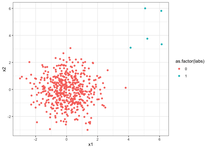
We will use 3 methods from the DDoutlier package, KNN, LOF and COF. We will compute the outlier scores and use the area under the Receiver Operator Characteristic (ROC) Curve to see the accuracy of these methods.
set.seed(1)
X1 <- data.frame(x1=rnorm(500), x2=rnorm(500))
oo <- data.frame(x1=rnorm(5, mean=5), x2=rnorm(5, mean=5))
X <- rbind.data.frame(X1, oo)
labs <- c(rep(0, 500), rep(1, 5))
X <- cbind.data.frame(X, labs)

ggplot(X, aes(x=x1, y=x2, color=as.factor(labs))) + geom_point() + theme_bw()

# Outlier Detection Methods
knn_scores <- DDoutlier::KNN_AGG(X)
lof_scores <- DDoutlier::LOF(X)
cof_scores <- DDoutlier::COF(X)

# ROC Curve
knn_roc <- pROC::roc(labs, knn_scores)
## Setting levels: control = 0, case = 1
## Setting direction: controls < cases
knn_roc
##
## Call:
## roc.default(response = labs, predictor = knn_scores)
##
## Data: knn_scores in 500 controls (labs 0) < 5 cases (labs 1).
## Area under the curve: 1
lof_roc <- pROC::roc(labs, lof_scores)
## Setting levels: control = 0, case = 1
## Setting direction: controls < cases
lof_roc
##
## Call:
## roc.default(response = labs, predictor = lof_scores)
##
## Data: lof_scores in 500 controls (labs 0) < 5 cases (labs 1).
## Area under the curve: 0.9884
cof_roc <- pROC::roc(labs, cof_scores)
## Setting levels: control = 0, case = 1
## Setting direction: controls < cases
cof_roc
##
## Call:
## roc.default(response = labs, predictor = cof_scores)
##
## Data: cof_scores in 500 controls (labs 0) < 5 cases (labs 1).
## Area under the curve: 0.8212
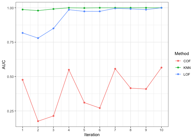
This example had rather obvious outliers. Next, we look at the case when outliers slowly move out from the main distribution. To do this, we consider several iterations of the same experiment. For the first iteration, the outliers are at the boundary of the normal distribution. With each iteration, the outliers move out, bit by bit. We do this with a parameter $\mu$, that starts at 2 and increases by 0.5 in each iteration. Which method gives better performance then?
set.seed(1)
knn_auc <- lof_auc <- cof_auc <- rep(0, 10)
for(i in 1:10){
  X1 <- data.frame(x1=rnorm(500), x2=rnorm(500))
  mu <- 2 + (i-1)/2
  oo <- data.frame(x1=rnorm(5, mean=mu, sd=0.2), x2=rnorm(5, mean=mu, sd=0.2))
  X <- rbind.data.frame(X1, oo)
  labs <- c(rep(0, 500), rep(1, 5))
  X <- cbind.data.frame(X, labs)

  # Outlier Detection Methods
  knn_scores <- DDoutlier::KNN_AGG(X)
  lof_scores <- DDoutlier::LOF(X)
  cof_scores <- DDoutlier::COF(X)

  # Area Under ROC = AUC values
  # KNN
  roc_obj <- pROC::roc(labs, knn_scores, direction ="<")
  knn_auc[i] <- roc_obj$auc

  # LOF
  roc_obj <- pROC::roc(labs, lof_scores, direction ="<")
  lof_auc[i] <- roc_obj$auc

  # COF
  roc_obj <- pROC::roc(labs, cof_scores, direction ="<")
  cof_auc[i] <- roc_obj$auc
}
## Setting levels: control = 0, case = 1
## Setting levels: control = 0, case = 1
## Setting levels: control = 0, case = 1
## Setting levels: control = 0, case = 1
## Setting levels: control = 0, case = 1
## Setting levels: control = 0, case = 1
## Setting levels: control = 0, case = 1
## Setting levels: control = 0, case = 1
## Setting levels: control = 0, case = 1
## Setting levels: control = 0, case = 1
## Setting levels: control = 0, case = 1
## Setting levels: control = 0, case = 1
## Setting levels: control = 0, case = 1
## Setting levels: control = 0, case = 1
## Setting levels: control = 0, case = 1
## Setting levels: control = 0, case = 1
## Setting levels: control = 0, case = 1
## Setting levels: control = 0, case = 1
## Setting levels: control = 0, case = 1
## Setting levels: control = 0, case = 1
## Setting levels: control = 0, case = 1
## Setting levels: control = 0, case = 1
## Setting levels: control = 0, case = 1
## Setting levels: control = 0, case = 1
## Setting levels: control = 0, case = 1
## Setting levels: control = 0, case = 1
## Setting levels: control = 0, case = 1
## Setting levels: control = 0, case = 1
## Setting levels: control = 0, case = 1
## Setting levels: control = 0, case = 1
df <- data.frame(Iteration=1:10, KNN=knn_auc, LOF=lof_auc, COF=cof_auc)
dfl <- tidyr::pivot_longer(df, 2:4)
colnames(dfl)[2:3] <- c("Method", "AUC")
ggplot(dfl, aes(x=Iteration, y=AUC, color=Method)) + geom_point() + geom_line() + scale_x_continuous(breaks=1:10) + theme_bw()

KNN is performing better than LOF. COF is not performing well at all. Maybe the parameters are not suitable for COF. Is KNN significantly better than LOF? To answer that question, we can repeat this example $n$ times and analyse the results.
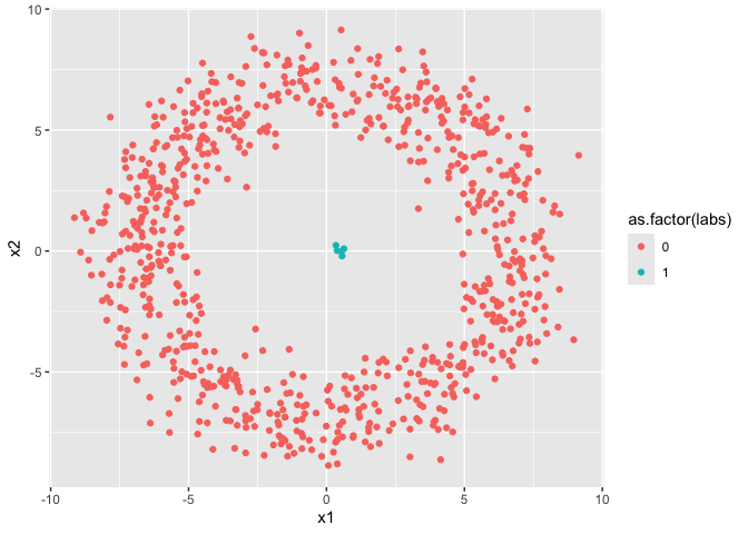
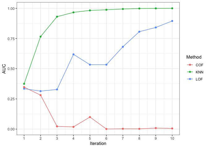
Let us consider another example. In this one, the points live in an annulus and the outliers are moving into the hole in each iteration.
set.seed(1)
r1 <-runif(805)
r2 <-rnorm(805, mean=5)
theta = 2*pi*r1;
R1 <- 2
R2 <- 2
dist = r2+R2;
x =  dist * cos(theta)
y =  dist * sin(theta)

X <- data.frame(
    x1 = x,
    x2 = y
)
labs <- c(rep(0,800), rep(1,5))
nn <- dim(X)[1]
knn_auc <- lof_auc <- cof_auc <- rep(0, 10)
for(i in 1:10){
  mu <-  5 - (i-1)*0.5
  z <- cbind(rnorm(5,mu, sd=0.2), rnorm(5,0, sd=0.2))
  X[801:805, 1:2] <- z

  # Outlier Detection Methods
  knn_scores <- DDoutlier::KNN_AGG(X)
  lof_scores <- DDoutlier::LOF(X)
  cof_scores <- DDoutlier::COF(X)

  # Area Under ROC = AUC values
  # KNN
  roc_obj <- pROC::roc(labs, knn_scores, direction ="<")
  knn_auc[i] <- roc_obj$auc

  # LOF
  roc_obj <- pROC::roc(labs, lof_scores, direction ="<")
  lof_auc[i] <- roc_obj$auc

  # COF
  roc_obj <- pROC::roc(labs, cof_scores, direction ="<")
  cof_auc[i] <- roc_obj$auc
}
## Setting levels: control = 0, case = 1
## Setting levels: control = 0, case = 1
## Setting levels: control = 0, case = 1
## Setting levels: control = 0, case = 1
## Setting levels: control = 0, case = 1
## Setting levels: control = 0, case = 1
## Setting levels: control = 0, case = 1
## Setting levels: control = 0, case = 1
## Setting levels: control = 0, case = 1
## Setting levels: control = 0, case = 1
## Setting levels: control = 0, case = 1
## Setting levels: control = 0, case = 1
## Setting levels: control = 0, case = 1
## Setting levels: control = 0, case = 1
## Setting levels: control = 0, case = 1
## Setting levels: control = 0, case = 1
## Setting levels: control = 0, case = 1
## Setting levels: control = 0, case = 1
## Setting levels: control = 0, case = 1
## Setting levels: control = 0, case = 1
## Setting levels: control = 0, case = 1
## Setting levels: control = 0, case = 1
## Setting levels: control = 0, case = 1
## Setting levels: control = 0, case = 1
## Setting levels: control = 0, case = 1
## Setting levels: control = 0, case = 1
## Setting levels: control = 0, case = 1
## Setting levels: control = 0, case = 1
## Setting levels: control = 0, case = 1
## Setting levels: control = 0, case = 1
X <- cbind.data.frame(X, labs)
# Plot of points in the last iteration
ggplot(X, aes(x1, x2, col=as.factor(labs))) + geom_point()

df <- data.frame(Iteration=1:10, KNN=knn_auc, LOF=lof_auc, COF=cof_auc)
dfl <- tidyr::pivot_longer(df, 2:4)
colnames(dfl)[2:3] <- c("Method", "AUC")
ggplot(dfl, aes(x=Iteration, y=AUC, color=Method)) + geom_point() + geom_line() + scale_x_continuous(breaks=1:10) + theme_bw()

We see that KNN > LOF > COF for this example. Again, by repeating the example many times, we can reduce the effect of randomness.
