Identifies outliers using the algorithm lookout.

This function identifies outliers using the algorithm lookout, an outlier detection method that uses leave-one-out kernel density estimates and generalized Pareto distributions to find outliers.

Usage

lookout(
  X,
  alpha = 0.01,
  beta = 0.9,
  gamma = 0.98,
  bw = NULL,
  gpd = NULL,
  scale = TRUE,
  fast = NROW(X) > 10000,
  old_version = FALSE
)

Arguments

X: The numerical input data in a data.frame, matrix or tibble format.
alpha: The level of significance. Default is 0.01. So there is a 1/100 chance of any point being falsely classified as an outlier.
beta: The quantile threshold used in the GPD estimation. Default is 0.90. To ensure there is enough data available, values greater than 0.90 are set to 0.90.
gamma: The quantile of the minimum spanning tree edge lengths used to compute the bandwidth. Default is 0.98. Ignored if bw is provided, and ignored when old_version = TRUE, where the largest gap between consecutive edge lengths is used instead. See Details.
bw: The support radius of the Epanechnikov kernel, on the scale of the data after any scaling. If NULL (default), it is computed from the minimum spanning tree of the data as described in Details.
gpd: Generalized Pareto distribution parameters. If NULL (the default), these are estimated from the data.
scale: If TRUE (the default), the data are scaled before the bandwidth and density estimates are computed: with mvscale() when old_version = FALSE, so that the columns are approximately uncorrelated with unit scale, or by scaling each column to the range [0, 1] when old_version = TRUE.
fast: If TRUE, each kernel density estimate is a sum over the k nearest neighbours of the point only, including the point itself, where k = min(max(ceiling(n / 200), 100), n, 500) and n = NROW(X); so k is between 100 and 500, and equals 100 whenever 100 <= n <= 20000. Wherever more than k - 1 other observations lie inside the kernel support, which is typical in the bulk of the data in three or more dimensions, the sum is truncated and the estimate is lower than the exact one. Sparse observations, which are the candidates for outliers, have fewer than k neighbours inside the support and their estimates are unchanged, although the GPD threshold and fit can still differ. If FALSE, each kernel is summed over exactly the observations inside its support, found with a fixed-radius search (frNN()). The time and memory of this exact computation are proportional to the number of pairs of observations within bw of each other. In two dimensions this is usually modest, but in three or more dimensions the kernel support in the bulk of the data can contain thousands of observations, so the exact computation is still of order n^2 in the worst case and fast = TRUE remains the practical choice for large n. Default is TRUE when NROW(X) > 10000. The bandwidth calculation always uses all of the data.
old_version: If TRUE, the algorithm of Kandanaarachchi and Hyndman (2022) is used. Default is FALSE, giving the algorithm of Hyndman, Kandanaarachchi and Turner (2026). See Details.

Value

A list with the following components:

data: The input data X, before any scaling.
outliers: The set of outliers.
outlier_probability: The GPD probability of the data.
outlier_scores: The outlier scores of the data.
bandwidth: The support radius of the Epanechnikov kernel: either bw, or the value computed from the minimum spanning tree multiplied by sqrt(NCOL(X) + 4).
kde: The kernel density estimate values.
lookde: The leave-one-out kde values.
gpd: The fitted GPD parameters.
call: The matched call.

Details

The algorithm has three steps.

Scaling. When scale = TRUE, the data are first scaled with mvscale(): each column is centred at its median, and the data are rotated and scaled using the Cholesky factor of the inverse of a robust (MCD) covariance estimate, so that the columns are approximately uncorrelated with unit scale.

Leave-one-out density estimates. A kernel density estimate is computed at each observation using a spherically symmetric Epanechnikov kernel with support radius bw, and the contribution of the observation itself is then removed to give a leave-one-out estimate. When bw = NULL, the bandwidth is computed from the Euclidean minimum spanning tree of the (scaled) data by find_tda_bw(): the gamma quantile (type 8) of the tree's edge lengths is multiplied by sqrt(m + 4), where m = NCOL(X). A spherically symmetric Epanechnikov kernel with support radius h in m dimensions has standard deviation h / sqrt(m + 4) in each coordinate, so this scaling makes the kernel's per-coordinate standard deviation equal to the quantile. When fast = TRUE, each kernel is summed over the k nearest neighbours of the point only; see the fast argument.

Extreme value model. The negative logarithms of the density estimates (the surprisals) above their beta quantile are modelled with a generalized Pareto distribution (GPD), fitted by maximum likelihood using fpot(). Because the surprisals are bounded, the shape parameter is constrained to be at most zero: if the unconstrained estimate is positive, the GPD is refitted with the shape fixed at zero. The fitted GPD gives, for each observation, the probability of a leave-one-out surprisal at least as large as the one observed, multiplied by 1 - beta. Observations whose probability is below alpha are declared outliers.

Setting old_version = TRUE gives the algorithm of Kandanaarachchi and Hyndman (2022) instead. It differs in three places: the data are scaled so that each column lies in [0, 1], rather than with mvscale(); the bandwidth is the lower end of the largest gap between consecutive minimum spanning tree edge lengths among those at or above their median, rather than the gamma quantile, again multiplied by sqrt(m + 4); and the GPD shape parameter is not constrained.

References

Kandanaarachchi, S, and Hyndman, RJ (2022) Leave-one-out kernel density estimates for outlier detection, J Computational & Graphical Statistics, 31(2), 586-599. https://robjhyndman.com/publications/lookout/.

Hyndman, RJ, Kandanaarachchi, S, and Turner, K (2026) Lookout 2: Anomaly detection via leave-one-out kernel density estimation, arXiv:2603.22636. https://robjhyndman.com/publications/lookout2.html

Examples

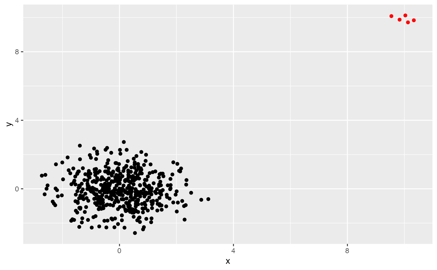
X <- rbind(
  data.frame(
    x = rnorm(500),
    y = rnorm(500)
  ),
  data.frame(
    x = rnorm(5, mean = 10, sd = 0.2),
    y = rnorm(5, mean = 10, sd = 0.2)
  )
)
lo <- lookout(X)
lo
#> Leave-out-out KDE outliers using lookout algorithm
#> 
#> Call: lookout(X = X)
#> 
#>    Outliers  Probability
#> 1        78 0.0021870275
#> 2       128 0.0006773301
#> 3       219 0.0086577418
#> 4       221 0.0000000000
#> 5       305 0.0066487886
#> 6       435 0.0036292648
#> 7       501 0.0059291894
#> 8       502 0.0052703980
#> 9       503 0.0059618874
#> 10      504 0.0043944614
#> 11      505 0.0059026768
#> 
autoplot(lo)