Computes outlier persistence for a range of significance values.

This function computes outlier persistence for a range of significance values, using the algorithm lookout, an outlier detection method that uses leave-one-out kernel density estimates and generalized Pareto distributions to find outliers.

Usage

persisting_outliers(
  X,
  alpha = seq(0.01, 0.1, by = 0.01),
  st_qq = 0.9,
  scale = TRUE,
  num_steps = 20,
  old_version = FALSE
)

Arguments

X

The input data in a matrix, data.frame, or tibble format. All columns should be numeric.

alpha

Grid of significance levels.

st_qq

The quantile of the minimum spanning tree edge lengths at which the bandwidth sequence starts. The sequence ends at the largest edge length. Both are multiplied by sqrt(NCOL(X) + 4) to give the support radius of the Epanechnikov kernel; see find_tda_bw().

scale

If TRUE, the data is scaled. Default is TRUE. Which scaling method is used depends on the old_version parameter. See lookout for details.

num_steps

The length of the bandwidth sequence.

old_version

Logical indicator of which version of the algorithm to use.

Value

A list with the following components:

out

A 3D array of N x num_steps x num_alpha where N denotes the number of observations, num_steps denote the length of the bandwidth sequence, and num_alpha denotes the number of significance levels. This is a binary array and the entries are set to 1 if that observation is an outlier for that particular bandwidth and significance level.

bw

The set of bandwidth values.

gpdparas

The GPD parameters used.

lookoutbw

The bandwidth used for the GPD fit: the lower end of the largest gap between consecutive minimum spanning tree edge lengths among those at or above their median (the rule used by lookout() when old_version = TRUE), multiplied by sqrt(NCOL(X) + 4).

Examples

X <- rbind(
  data.frame(
    x = rnorm(500),
    y = rnorm(500)
  ),
  data.frame(
    x = rnorm(5, mean = 10, sd = 0.2),
    y = rnorm(5, mean = 10, sd = 0.2)
  )
)
plot(X, pch = 19)

outliers <- persisting_outliers(X, scale = FALSE)
outliers
#> Persistent outliers using lookout algorithm
#> 
#> Call: persisting_outliers(X = X, scale = FALSE)
#> 
#> Lookout bandwidth:  2.861997 
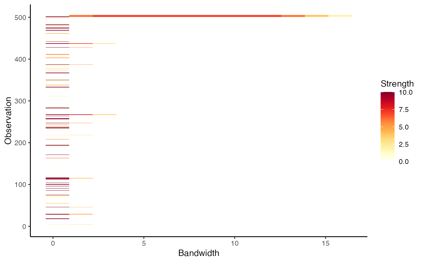
autoplot(outliers)