The R package netseer

netseer

The goal of netseer is to predict the graph structure including new nodes and edges from a time series of graphs. The methodology is explained in the preprint (Kandanaarachchi et al. 2025). We will illustrate an example in this vignette.

Installation

You can install the development version of netseer from GitHub with:

# install.packages("devtools")
devtools::install_github("sevvandi/netseer")

An example

This is a basic example which shows you how to predict a graph at the next time point. First let us generate some graphs.

library(netseer)
library(igraph)
#> 
#> Attaching package: 'igraph'
#> The following objects are masked from 'package:stats':
#> 
#>     decompose, spectrum
#> The following object is masked from 'package:base':
#> 
#>     union

set.seed(2024)
edge_increase_val <- new_nodes_val <- del_edge_val <- 0.1
graphlist <- list()
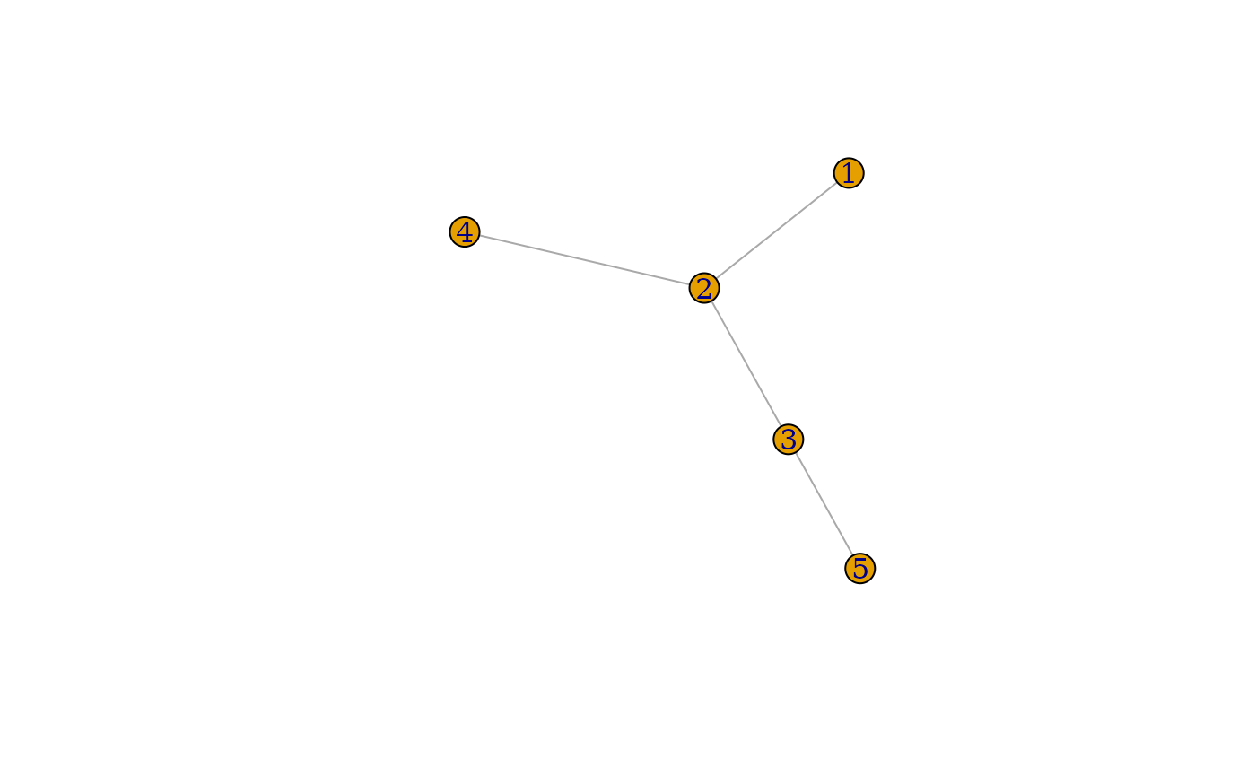
graphlist[[1]] <- gr <-  igraph::sample_pa(5, directed = FALSE)
for(i in 2:15){
gr <-  generate_graph_exp(gr,
                          del_edge = del_edge_val,
                          new_nodes = new_nodes_val,
                          edge_increase = edge_increase_val )
graphlist[[i]] <- gr
}

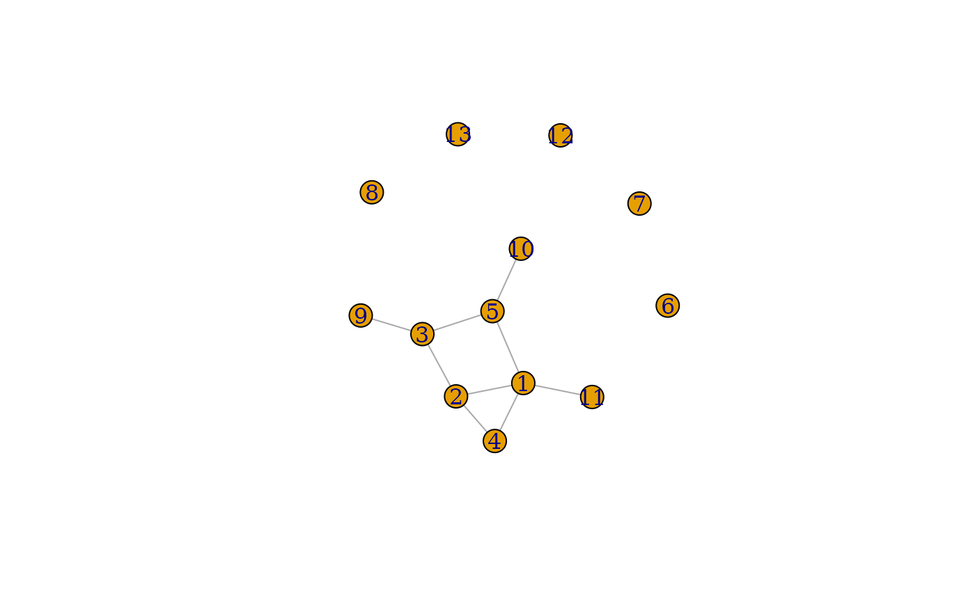
The graphlist contains the list of graphs we generated. Each graph is an igraph object. Let’s plot a couple of them.

Plotting a couple of graphs

plot(graphlist[[1]])

plot(graphlist[[8]])

plot(graphlist[[15]])

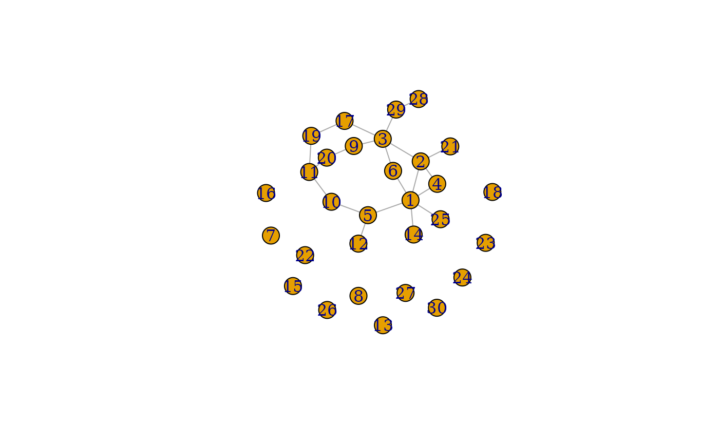
Predicting the next graph

Let’s predict the next graph. The argument $h = 1$ specifies we want to predict the graph at the next time point.

grpred <- predict_graph(graphlist[1:15],h = 1)
#> Registered S3 method overwritten by 'tsibble':
#>   method               from 
#>   as_tibble.grouped_df dplyr
#> Warning: 2 errors (1 unique) encountered for arima
#> [2] missing value where TRUE/FALSE needed
#> Registered S3 method overwritten by 'quantmod':
#>   method            from
#>   as.zoo.data.frame zoo
grpred
#> $graph_mean
#> IGRAPH 1df11f7 U--- 34 23 -- 
#> + edges from 1df11f7:
#>  [1] 28--29 17--19 11--20 11--19 10--11  9--20  5--12  5--10  3--29  3--17
#> [11]  3-- 9  3-- 6  3-- 5  2--21  2--17  2-- 4  2-- 3  1--25  1--14  1-- 6
#> [21]  1-- 5  1-- 4  1-- 2
#> 
#> $graph_lower
#> NULL
#> 
#> $graph_upper
#> NULL

plot(grpred$graph_mean)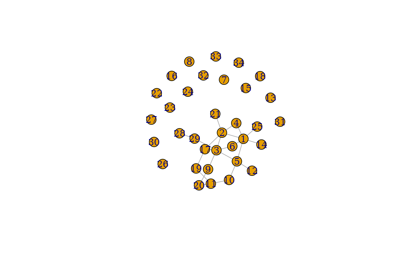

ecount(grpred$graph_mean)
#> [1] 23
vcount(grpred$graph_mean)
#> [1] 34

Predicting the graph at 2 time steps ahead

Now let us predict the graph at 2 time steps ahead with $h=2$.

grpred2 <- predict_graph(graphlist[1:15], h = 2)
#> Warning: 2 errors (1 unique) encountered for arima
#> [2] missing value where TRUE/FALSE needed
grpred2
#> $graph_mean
#> IGRAPH 0441afc U--- 37 26 -- 
#> + edges from 0441afc:
#>  [1] 28--29 17--19 13--15 11--20 11--19 10--11  9--20  5--12  5--10  4-- 7
#> [11]  3--29  3--17  3-- 9  3-- 6  3-- 5  2--21  2--17  2-- 4  2-- 3  1--25
#> [21]  1--14  1--11  1-- 6  1-- 5  1-- 4  1-- 2
#> 
#> $graph_lower
#> NULL
#> 
#> $graph_upper
#> NULL

plot(grpred2$graph_mean)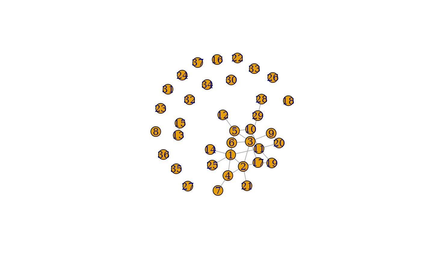

ecount(grpred2$graph_mean)
#> [1] 26
vcount(grpred2$graph_mean)
#> [1] 37

We see the predicted graph at $h=2$ has more vertices and edges than the graph at $h=1$.

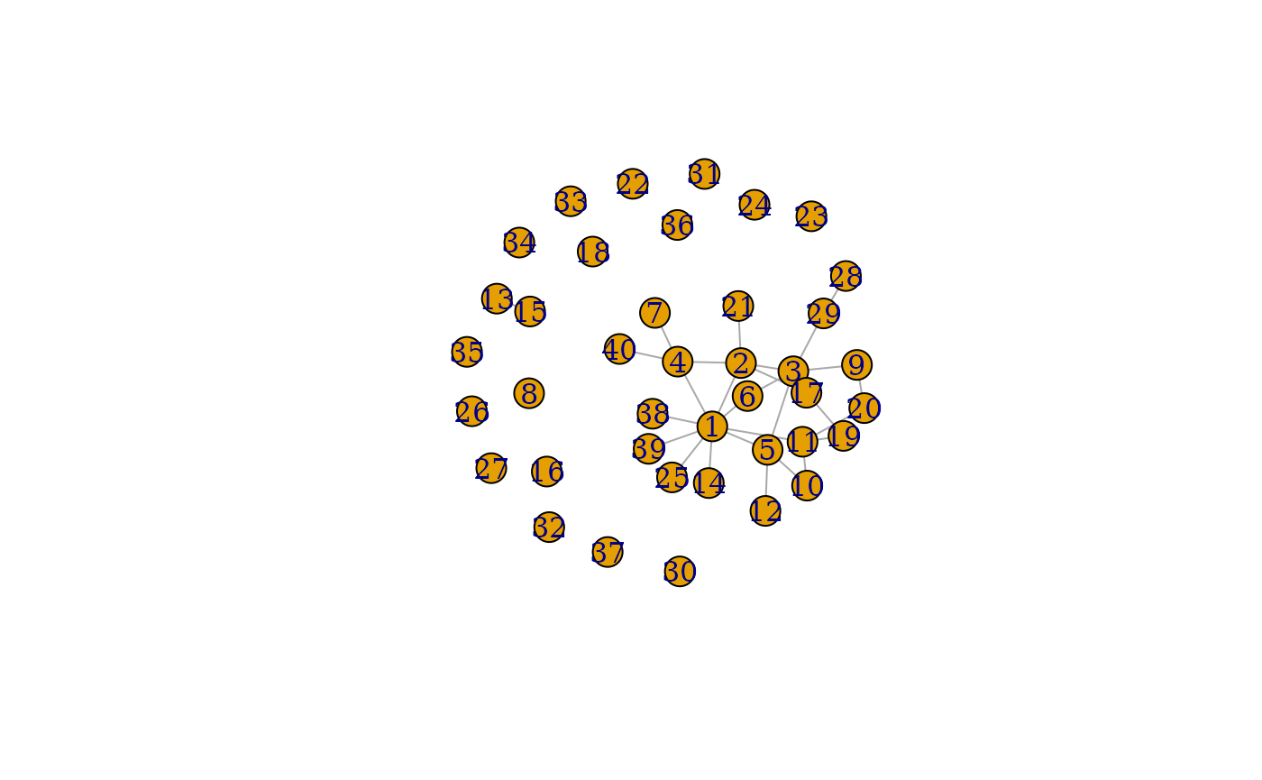
Predicting the graph at 3 time steps ahead

Similarly, we can predict the graph at 3 time steps ahead. We don’t have a limit on $h$. But generally, as we get further into the future, the predictions are less accurate. This is with everything, not just graphs.

grpred3 <- predict_graph(graphlist[1:15], h = 3)
#> Warning: 2 errors (1 unique) encountered for arima
#> [2] missing value where TRUE/FALSE needed
grpred3
#> $graph_mean
#> IGRAPH c6cf6e5 U--- 40 29 -- 
#> + edges from c6cf6e5:
#>  [1] 28--29 17--19 13--15 11--20 11--19 10--11  9--20  5--12  5--10  4-- 7
#> [11]  3--29  3--17  3-- 9  3-- 6  3-- 5  2--21  2--17  2-- 4  2-- 3  1--25
#> [21]  1--14  1--11  1-- 6  1-- 5  1-- 4  1-- 2  1--38  1--39  4--40
#> 
#> $graph_lower
#> NULL
#> 
#> $graph_upper
#> NULL

plot(grpred3$graph_mean)

ecount(grpred3$graph_mean)
#> [1] 29
vcount(grpred3$graph_mean)
#> [1] 40

References

Kandanaarachchi, Sevvandi, Ziqi Xu, Stefan Westerlund, and Conrad Sanderson. 2025. “Predicting Graph Structure via Adapted Flux Balance Analysis.” https://arxiv.org/abs/2507.05806.