Introducing Graphettes

library(igraph)
#> 
#> Attaching package: 'igraph'
#> The following objects are masked from 'package:stats':
#> 
#>     decompose, spectrum
#> The following object is masked from 'package:base':
#> 
#>     union
library(graphonmix)
library(ggplot2)

Graphettes are a graph generation methodology proposed in (Wijesinghe et al. 2026). A graphette has 3 components: a graphon $W$, a sequence $\{\rho_n\}_n$ and a graph edit function $f$. We can generate dense or sparse graphs from a graphette. On the sparse graph front, we can generate diverse sparse graphs, such as ring-added graphs that have bounded degree or graphs with large hubs like this social networks. We can generate trees as well. Let’s look at some examples.

Dense graphs from graphons and graphettes

Let’s start with a stochastic block model graphon.

mat <- matrix(c(0.9, 0.01, 0.02,
                0.01, 0.8, 0.03,
                0.02, 0.03, 0.7), nrow = 3, byrow = TRUE)
W <- sbm_graphon(mat, 100)
plot_graphon(W) +  coord_fixed(ratio = 1) 
#> Warning: Using `size` aesthetic for lines was deprecated in ggplot2 3.4.0.
#> ℹ Please use `linewidth` instead.
#> ℹ The deprecated feature was likely used in the graphonmix package.
#>   Please report the issue to the authors.
#> This warning is displayed once per session.
#> Call `lifecycle::last_lifecycle_warnings()` to see where this warning was
#> generated.

Using the graphon

Without using graphettes we can sample from this graphon as follows:

gr <- sample_graphon(W, 100)
plot(gr, vertex.size = 3, vertex.label = NA, main = "Graphon sampling")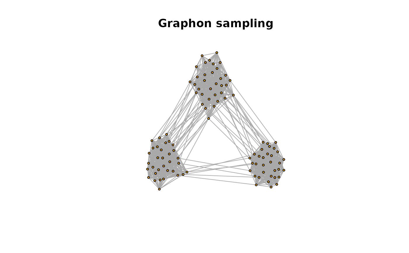

Using the graphette

To generate dense graphs from the graphette we set $\rho_n = 1$ for all $n$ and the graph edit function $f$ to the identity function. In the function call sample_graphette we set $\rho_n$ = NULL and graph_edit_function = NULL. That way, we get are actually sampling from the graphon $W$ without sparsifying it.

gr1 <- sample_graphette(W, n= 100)
plot(gr1, vertex.size = 3, vertex.label = NA, main = "Graphette sampling")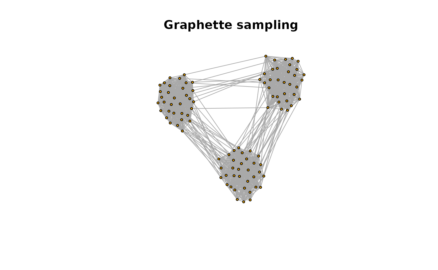

As you can see, in this instance sampling from the graphon or the graphette gives similar graphs.

Sparse graphs using $\rho_n$

Consider the same SBM graphon. We can sparsify it by considering $W_n = \rho_n W$ where $\rho_n \to 0$. And then we sample a graph $G_n$ with $n$ nodes from $W_n$. As $n \to \infty$ the edge density goes to zero making this graph sequence sparse. Let’s see how this works.

Using the standard graphon and $\rho_n$ separately

rho_n <- function(n) exp( -((n-100)/50 ))


W250 <- rho_n(250)*W
W300 <- rho_n(300)*W

gr1 <- sample_graphon(W, 100)
gr2 <- sample_graphon(W250, 250)
gr3 <- sample_graphon(W300, 300)


g1 <- plot_graphon(W) +  coord_fixed(ratio = 1) 
g2 <- plot_graphon(W250) +  coord_fixed(ratio = 1) 
g3 <- plot_graphon(W300) + coord_fixed(ratio = 1) 

gridExtra::grid.arrange(g1, g2, g3, nrow = 1)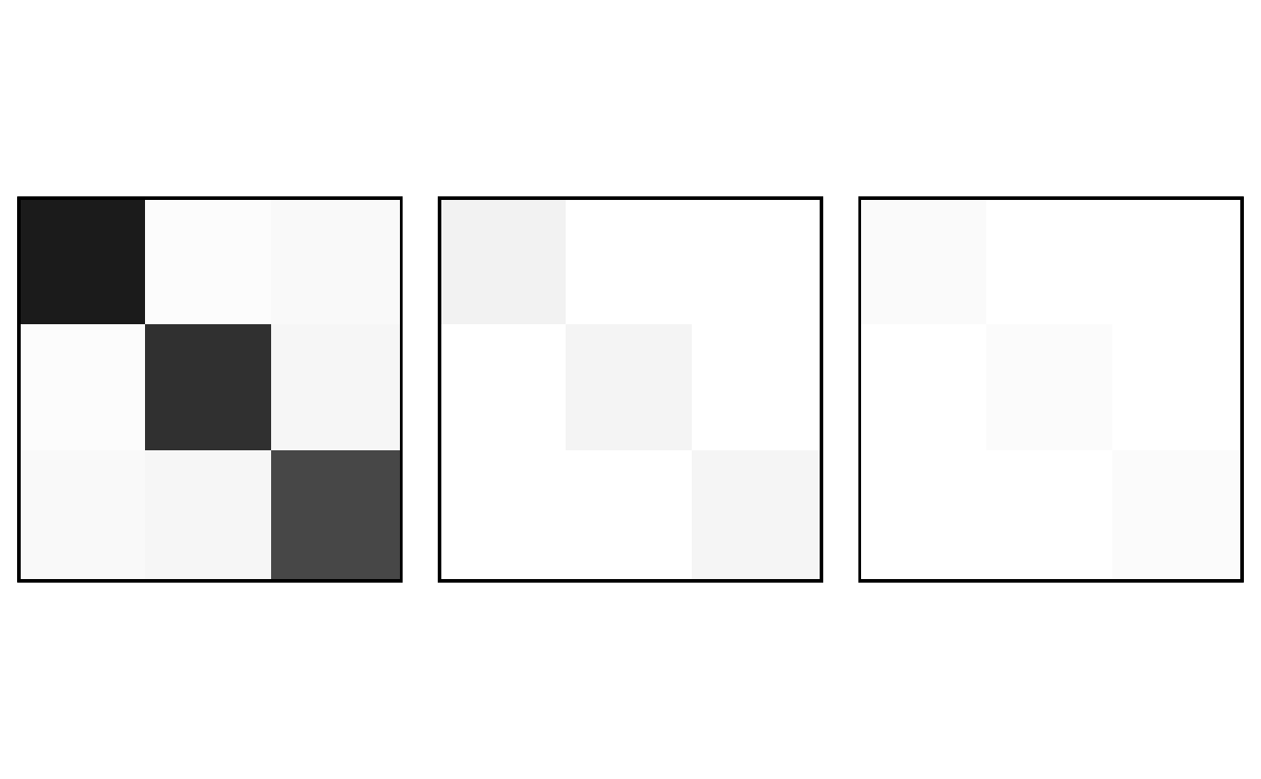

The three graphons are shown above and we see the colours get greyed out as $\rho_n$ goes to zero. Let’s plot the graphs sampled from the two graphons.

par(mfrow = c(1,3))
plot(gr1, vertex.size = 3, vertex.label = NA, main = "From W")
plot(gr2, vertex.size = 3, vertex.label = NA, main = "From W250")
plot(gr3, vertex.size = 3, vertex.label = NA, main = "From W300")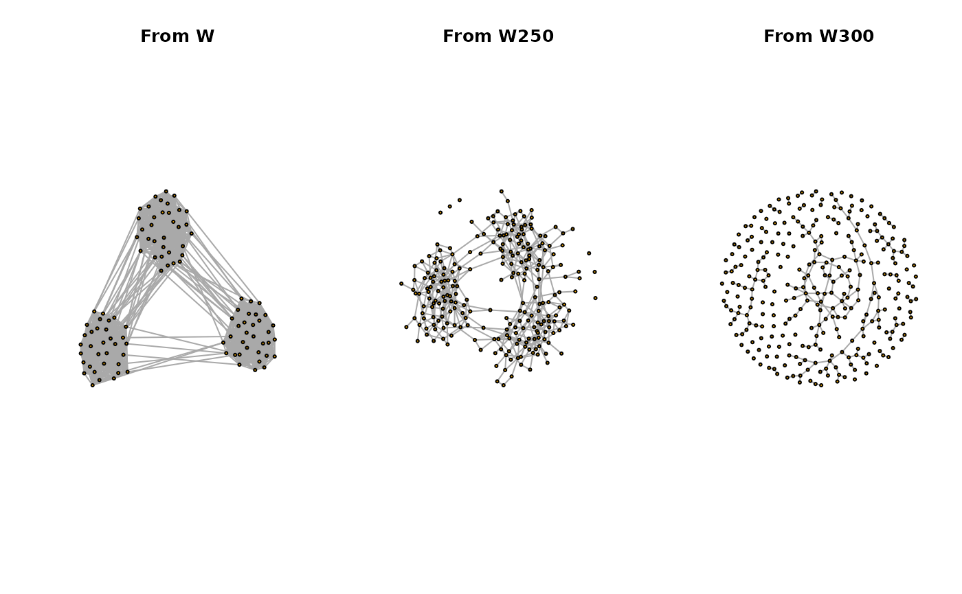

par(mfrow = c(1,1)) 

We see the graphs getting sparser.

Using the function sample_sparse_graphon

The function sample_sparse_graphon has a function parameter that can be used for $\rho_n$.

gr4 <- sample_sparse_graphon(W, rho_n, n = 250)
gr5 <- sample_sparse_graphon(W, rho_n, n = 300)

par(mfrow = c(1,2))
plot(gr4, vertex.size = 3, vertex.label = NA, main = "n = 250")
plot(gr5, vertex.size = 3, vertex.label = NA, main = "n = 300")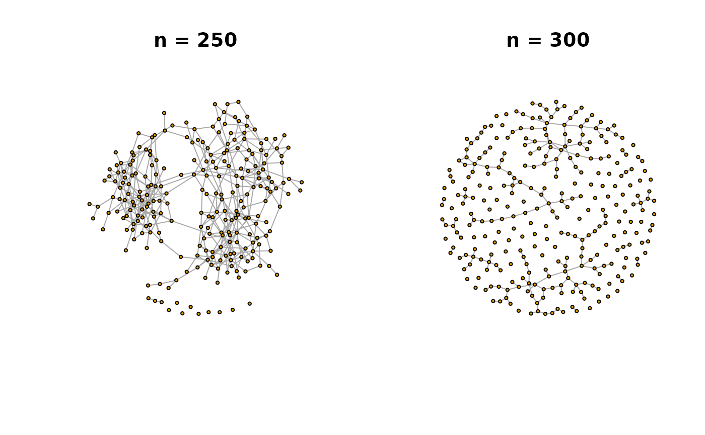

par(mfrow = c(1,1))

Using the graphette

We can use the sample_graphette to get the same functionality by setting *graph_edit_f = $NULL.

gr6 <- sample_graphette(W, rho_n, n = 250)
gr7 <- sample_graphette(W, rho_n, n = 300)


par(mfrow = c(1,2))
plot(gr6, vertex.size = 3, vertex.label = NA, main = "n = 250")
plot(gr7, vertex.size = 3, vertex.label = NA, main = "n = 300")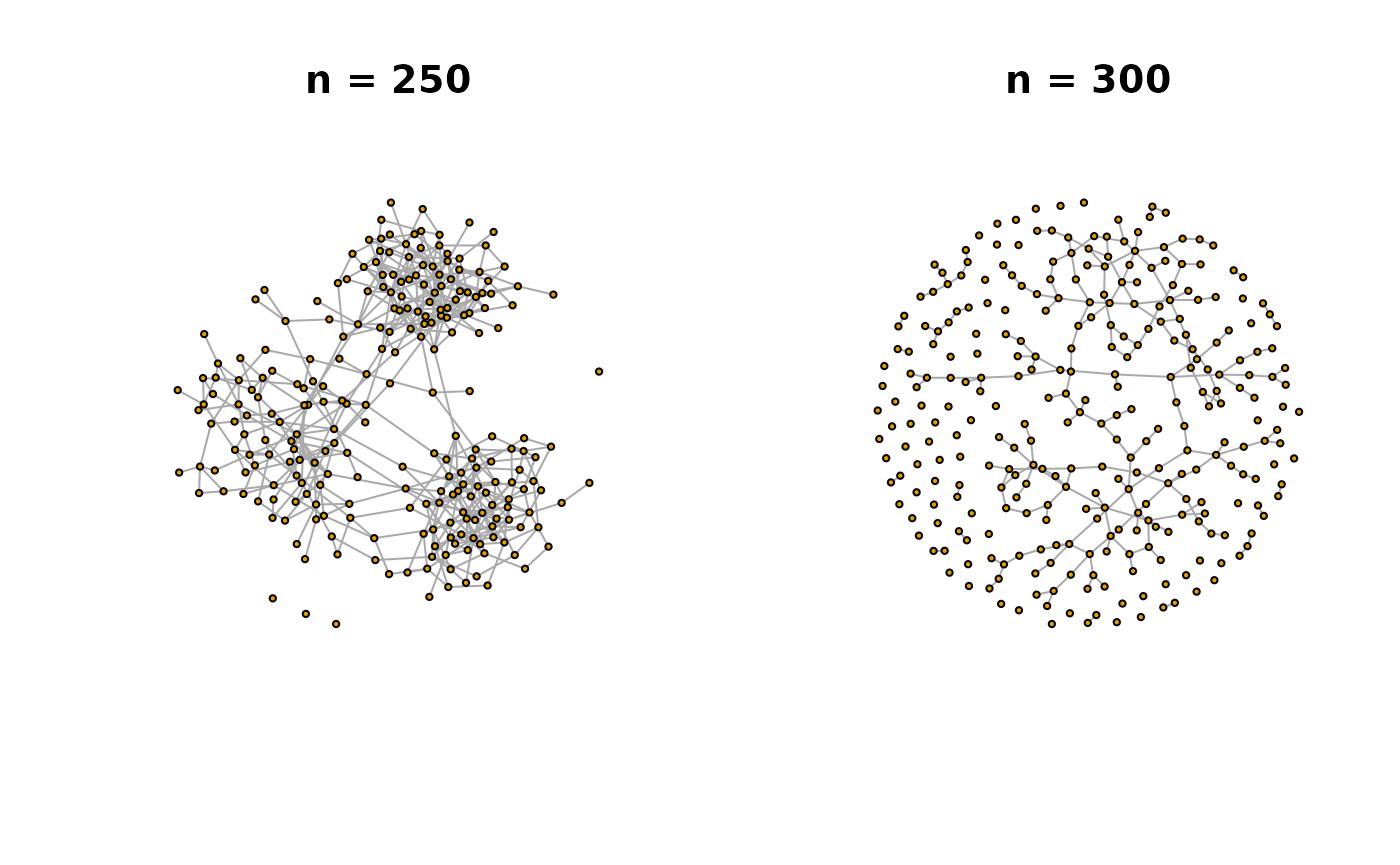

par(mfrow = c(1,1))

Sparse graphs using $\rho_n$ and the graph edit function

We have the functionality to add stars, add rings and remove cycles using the graph edit function.

Adding stars

The functions star_f1, star_f2, star_f3, star_f4 and star_f5 can be used to add stars. While there are slight differences, all of these functions use a Poisson process to add additional connections to each node. The parameter $t_or_p$ controls the intensity of the Poisson process.

gr8 <- sample_graphette(W, rho_n, "star_f1", n = 250, t_or_p = 2)
gr9 <- sample_graphette(W, rho_n, "star_f1", n = 300, t_or_p = 2)

par(mfrow = c(1,2))
plot(gr8, vertex.size = 3, vertex.label = NA, main = "n = 250")
plot(gr9, vertex.size = 3, vertex.label = NA, main = "n = 300")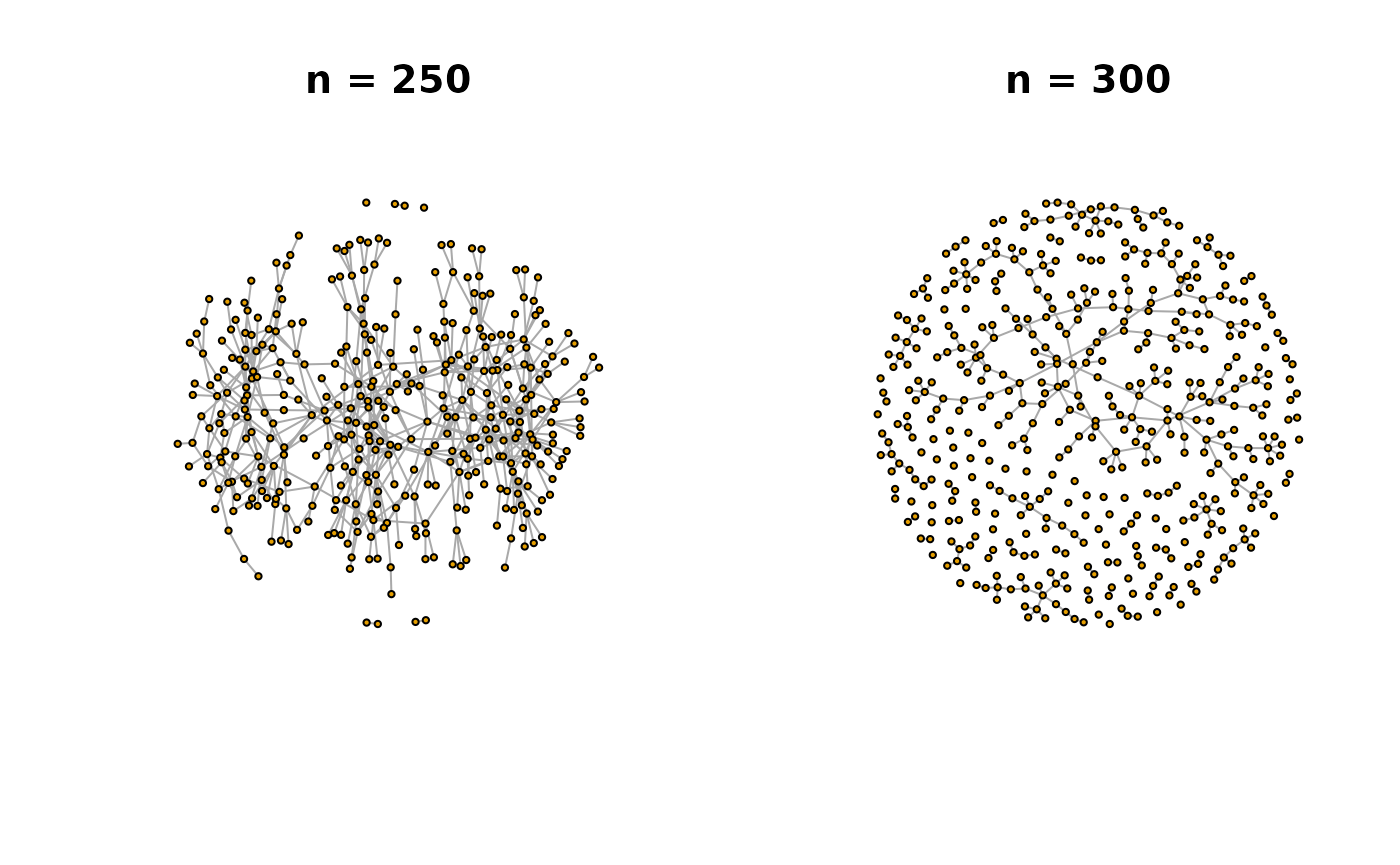

par(mfrow = c(1,1))

In the above example $\rho_n$ goes to 0 very fast. Let us use something a bit different

rho2 <- function(n)10/n
gr10 <- sample_graphette(W, rho2, "star_f1", n = 250, t_or_p = 2)
gr11 <- sample_graphette(W, rho2, "star_f1", n = 300, t_or_p = 2)

par(mfrow = c(1,2))
plot(gr10, vertex.size = 3, vertex.label = NA, main = "n = 250")
plot(gr11, vertex.size = 3, vertex.label = NA, main = "n = 300")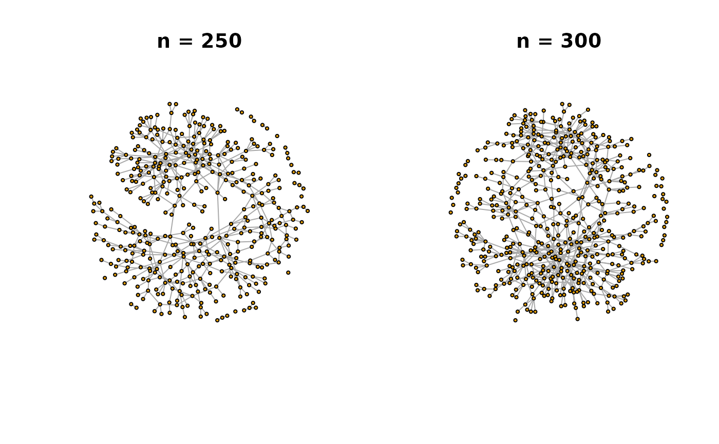

par(mfrow = c(1,1))

Adding rings

To add rings to the graph, use add_rings as the graph edit function. The parameter t_or_p gives the proportion of nodes to which rings are added. The default ring size is 5 or 6, but this can be changed.

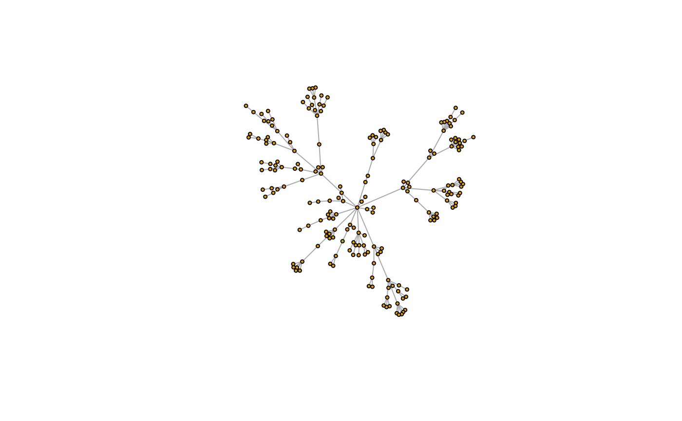
gr <- sample_graphette(W, rho_n, "add_rings", n = 100, t_or_p = 0.5, ring_sizes = c(10:15))

plot(gr, vertex.size = 3, vertex.label = NA)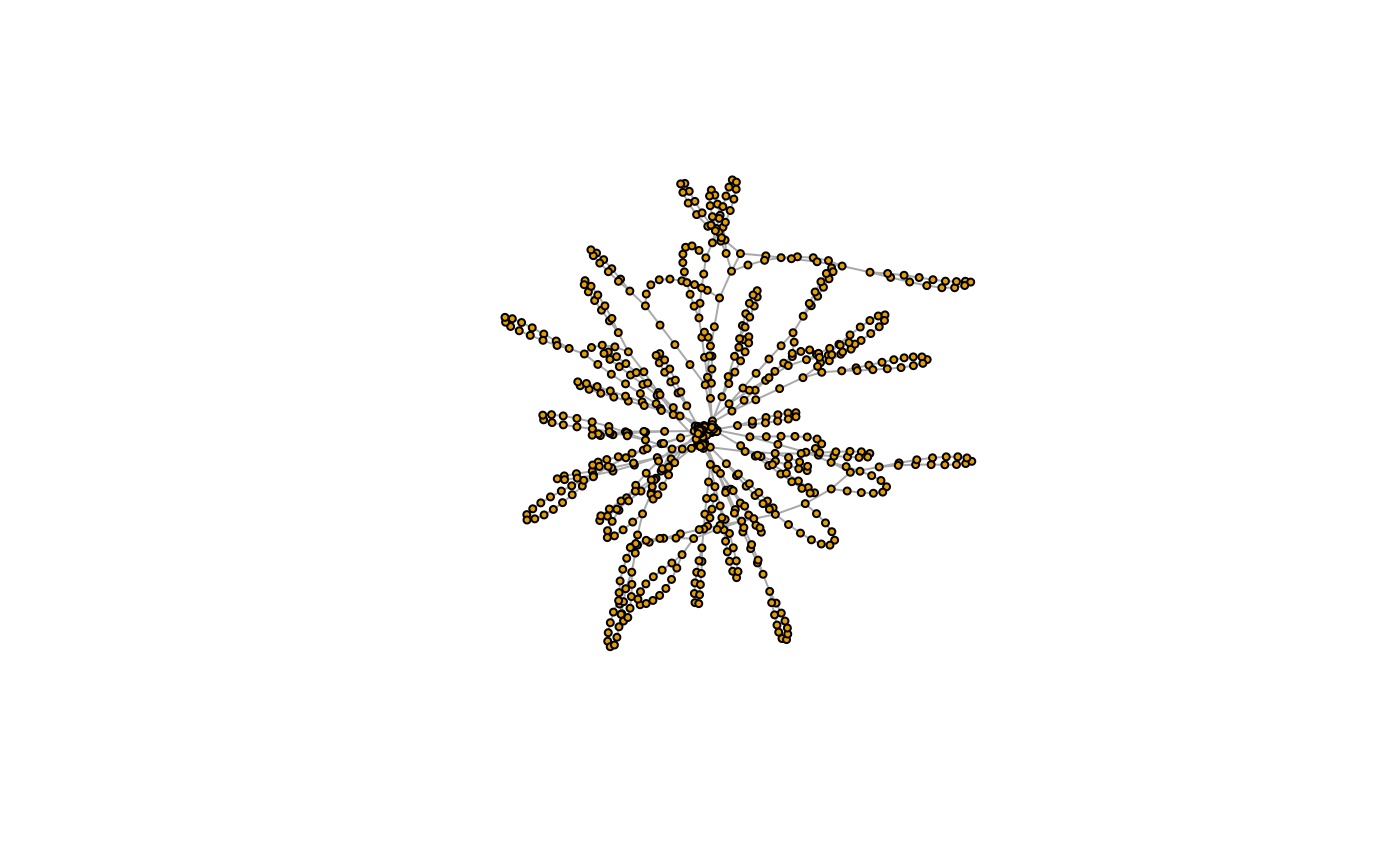

Removing cycles

To remove cycles from a graph, use remove_cycles as the graph edit function.

gr <- sample_graphette(W, rho_n, "remove_cycles", n = 200)

plot(gr, vertex.size = 3, vertex.label = NA)

References

Wijesinghe, Asiri, Sevvandi Kandanaarachchi, Daniel M Steinberg, and Cheng Soon Ong. 2026. “Flowette: Flow Matching with Graphette Priors for Graph Generation.” arXiv Preprint arXiv:2602.23566.