Sparse graphs from line graphons • graphonmix

library(graphonmix)
library(ggplot2)
library(igraph)
#> 
#> Attaching package: 'igraph'
#> The following objects are masked from 'package:stats':
#> 
#>     decompose, spectrum
#> The following object is masked from 'package:base':
#> 
#>     union
requireNamespace("gridExtra", quietly = TRUE)

Line graphs

Suppose $G$ is a graph. Then the line graph of $G$ , commonly denoted by $L(G)$ maps edges of $G$ to vertices of $L(G)$ and two vertices in $L(G)$ are connected if the original edges in $G$ share a common vertex. Here’s an example.

g1 <- make_star(4,mode = "undirected")
g1 <- add_vertices(g1, 1)
g1 <- add_edges(g1,c(4,5))

lg1 <- make_line_graph(g1)

par(mfrow = c(1,2))
plot(g1, vertex.label = NA, edge.label = c(1,2,3,4), main = "Graph G")
plot(lg1, vertex.label = c(1,2,3,4), vertex.size = 20, main = "Line graph L(G)")

Line graphs of star graphs

The key is that line graphs of stars are complete graphs. In the example below each edge of graph $G$ is a vertex in $L(G)$ . Two vertices in $L(G)$ are connected if the corresponding edges in $G$ share a vertex.

st <- make_star(10, mode = "undirected")
lgr_st <- make_line_graph(st)

par(mfrow = c(1,2))
plot(st, vertex.label = NA, main = "Star graph G")
plot(lgr_st, vertex.label = NA,  main = "Line graph L(G) of a st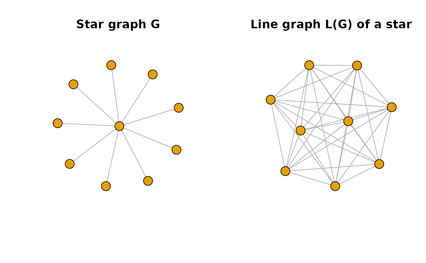ar")

Sparse graphs

A sequence of graphs is sparse if the edges grow subquadratically with the nodes. Star graphs are the ultimate sparse graphs, because a star of $n$ nodes has $n-1$ edges. A graph sequence is dense if the edges grow quadratically with the nodes. Erdos-Renyi graphs $G(n,p)$ with a fixed edge probability $p$ are dense. This can be seen from the edge density. Let’s generate a sequence of star graphs and a sequence of Erdos-Renyi graphs and see this in action.

stardensity <- gnpdensity <- rep(0, 20)
 
for(i in 1:20){
  n <- i*100
  gr1 <- sample_gnp(n, p = 0.1)
  gnpdensity[i] <- edge_density(gr1)
  gr2 <- make_star(n, mode = "undirected")
  stardensity[i] <- edge_density(gr2)
}
gnpdensity
#>  [1] 0.09696970 0.10120603 0.09895206 0.09996241 0.09983166 0.10017807
#>  [7] 0.09997956 0.09944931 0.10038561 0.09987988 0.10030275 0.09965388
#> [13] 0.09979392 0.10010926 0.09974917 0.10025094 0.09994807 0.09999568
#> [19] 0.10022560 0.10025063
stardensity
#>  [1] 0.020000000 0.010000000 0.006666667 0.005000000 0.004000000 0.003333333
#>  [7] 0.002857143 0.002500000 0.002222222 0.002000000 0.001818182 0.001666667
#> [13] 0.001538462 0.001428571 0.001333333 0.001250000 0.001176471 0.001111111
#> [19] 0.001052632 0.001000000

We see that the density of stars goes to zero whereas the density of GNP graphs hover around 0.1, because we have used the edge probability as 0.1.

Graphons

Graphons are graph limits. Suppose we have a graph $G$ . The empirical graphon of $G$ is when we scale the adjacency matrix to the unit square and color the small squares that correspond to ones in the adjacency matrix in black. Here we plot the empirical graphon of a star graph with 10 nodes.

gr <- make_star(10, mode = "undirected")
emp <- empirical_graphon(gr)
plot_graphon(emp) + coord_fixed()

Graphons of sparse graphs

The problem is graphons of sparse graphs are zero. Graphons are generally denoted by the letter $W$ . And if the graphs are sparse then $W = 0$ . That is, the empirical graphons converge to zero. Here, we’re a bit handwavy about convergence (actually, the convergence is with respect to the cut metric, but let’s let’s not discuss that).

gr <- make_star(20, mode = "undirected")
emp <- empirical_graphon(gr)
g1 <- plot_graphon(emp) + coord_fixed() + ggtitle('n = 10')

gr <- make_star(100, mode = "undirected") 
emp <- empirical_graphon(gr)
g2 <- plot_graphon(emp) + coord_fixed() + ggtitle('n = 100')

gr <- make_star(200, mode = "undirected")
emp <- empirical_graphon(gr)
g3 <- plot_graphon(emp) + coord_fixed() + ggtitle('n = 200')


gridExtra::grid.arrange(g1, g2, g3, nrow = 1)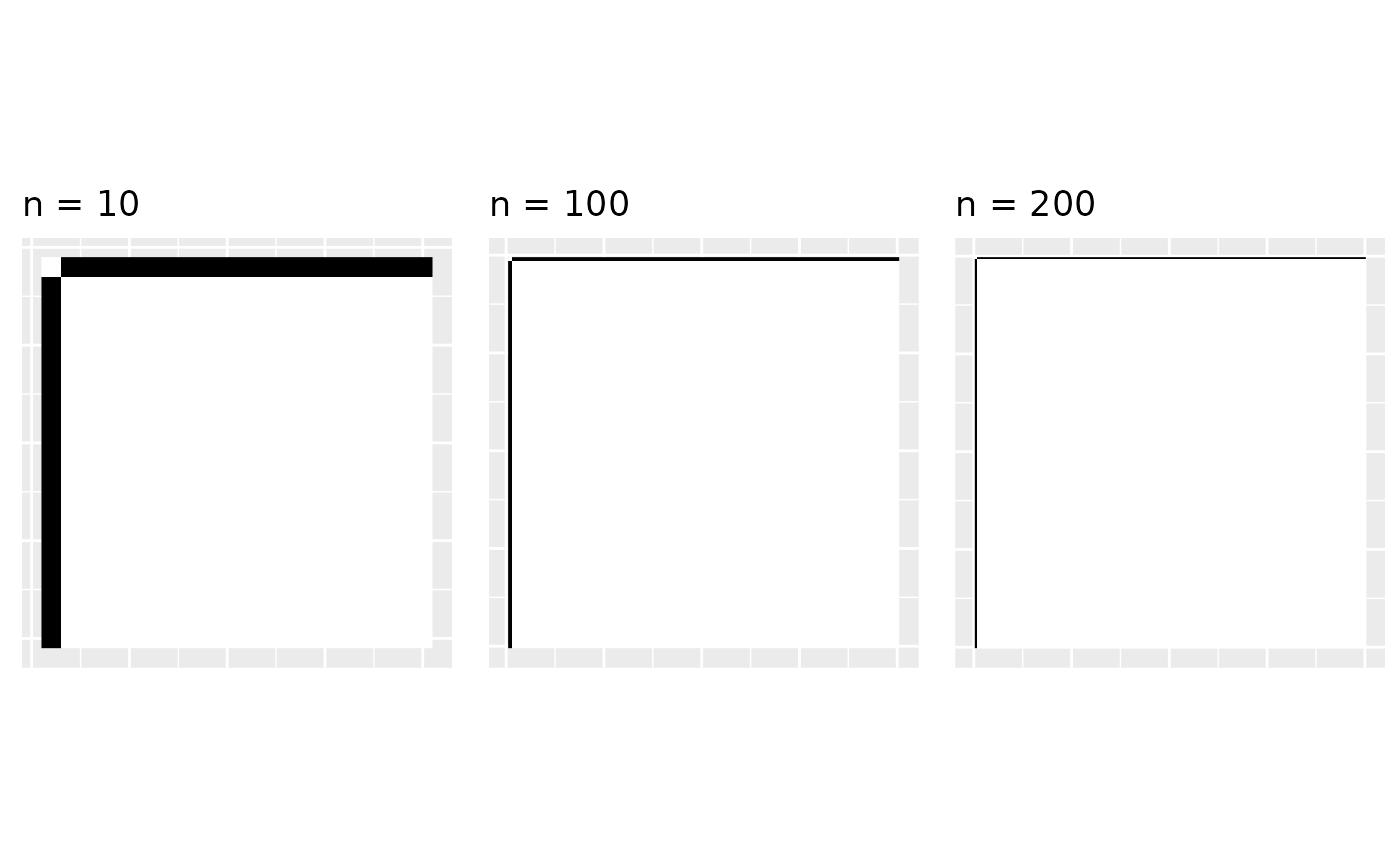

As $n \to \infty$ , there are less black parts in the empirical graphon and it converges to zero. When the graphon is zero, we cannot sample from it; it is not useful anymore. So what do we do?

Graphons of line graphs

For a subset of sparse graphs, such as the star graphs, their line graphs are dense. We discuss this in detail in (Kandanaarachchi and Ong 2024). The main example is star graphs.

gr1 <- make_star(10, mode = "undirected")
gr <- gr1 %du% gr1
lgr <- make_line_graph(gr)
emp <- empirical_graphon(lgr)
g1 <- plot_graphon(emp) + coord_fixed() + ggtitle('n = 20')


gr1 <- make_star(50, mode = "undirected")
gr <- gr1 %du% gr1
lgr <- make_line_graph(gr)
emp <- empirical_graphon(lgr)
g2 <- plot_graphon(emp) + coord_fixed() + ggtitle('n = 100')


gr1 <- make_star(100, mode = "undirected")
gr <- gr1 %du% gr1
lgr <- make_line_graph(gr)
emp <- empirical_graphon(lgr)
g3 <- plot_graphon(emp) + coord_fixed() + ggtitle('n = 200')


gridExtra::grid.arrange(g1, g2, g3, nrow = 1)

For the above example of two stars, the line graphs are dense and converge to a non-zero graphon.

Janson’s theorem

Janson (Janson 2016) proved that all line graph limits are disjoint clique graphs. This is a very important theorem for us because it tells us what the structure of line graph limits are. Janson explains that line graph limits can be written as a sequence of numbers $(p_1, p_2, \ldots)$ such that $\sum_i p_i \leq 1$ and $p_i \geq 0$ . The $p_i$ gives the width of each black box in the graphon.

Generating stars as inverse line graphs

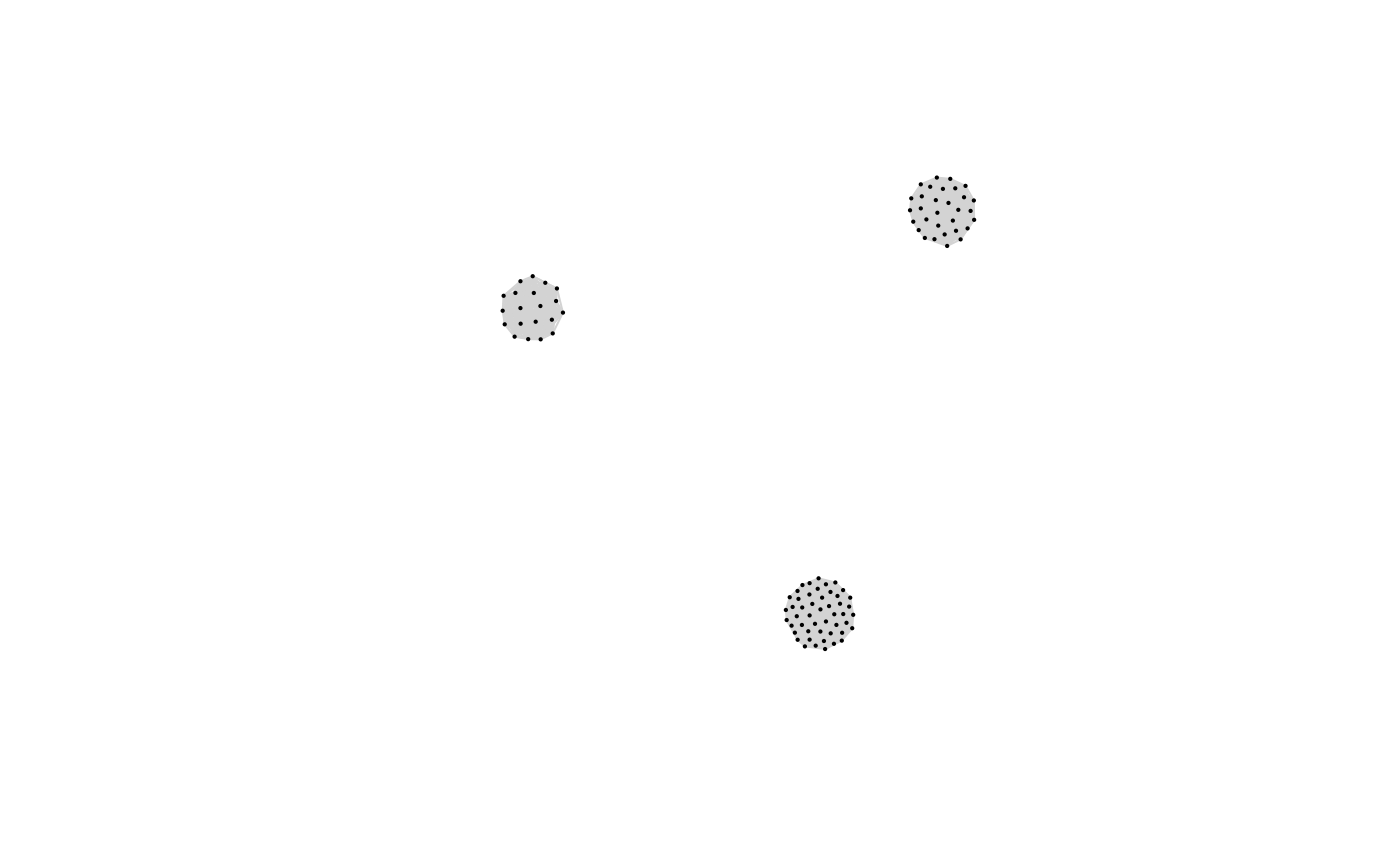
From a line graph limit we can generate a disjoint union of clique graphs like this.

wts <- c(0.5, 0.3, 0.2)
U <-  line_graphon(wts)
gr <- sample_graphon(U, n = 100)
plot(gr,
     vertex.size = 1,
     edge.color = "lightgray",     # Light colored edges
     vertex.label = NA,
     vertex.color = "lightblue"
)

The inverse line graphs of disjoint clique graphs are star graphs. And star graphs are sparse. We can generate star graphs using the weights or the partition $(p_1, p_2, \ldots)$ .

grsp <- generate_star_union(wts, n = 100)
plot(grsp,
     edge.curved = 0.3,
     vertex.size = 1,
     edge.color = "lightgray",     # Light colored edges
     vertex.label = NA,
     vertex.color = "lightblue"
)

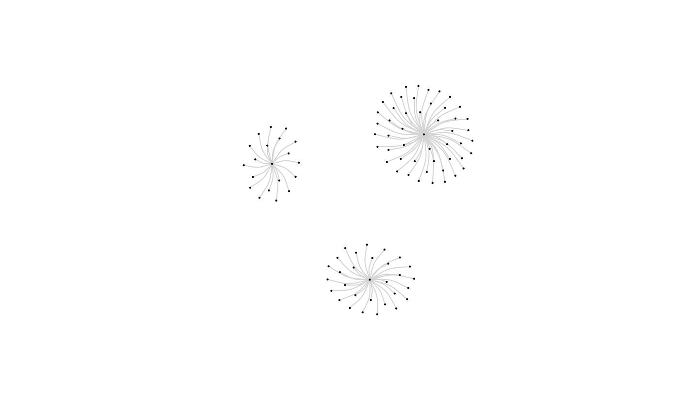
This is how the sparse part of the $(U,W)$ -mixture graph is generated. The vignette at Articles/Getting Started explains the mixture procedure.

References

Janson, Svante. 2016. “Graph Limits and Hereditary Properties.” European Journal of Combinatorics 52: 321–37.

Kandanaarachchi, Sevvandi, and Cheng Soon Ong. 2024. “Graphons of Line Graphs.” arXiv Preprint arXiv:2409.01656.